This is an introduction to TensorFlow written for some colleagues in October 2017. It assumes no prior knowledge of TensorFlow, but it is not a Deep Learning tutorial (and later parts assume that you know about DNNs). It covers everything from setting up TensorFlow on your machine to training and saving models. As a special feature, it covers how to efficiently use the recently introduced dataset API to load a training dataset given as single pictures. The tutorial is actually an interactive Jupyter notebook. You can download it here. It comes with the MNIST dataset as single pictures, so it is a bit heavy.
Installing TensorFlow & Jupyter Notebook
Before we get started, a few words on how to obtain a functioning TensorFlow installation. We will use Anaconda; this allows us to easily separate TensorFlow and its dependencies into a separate development environment. For this introduction, we will be using Python 2.7 and TensorFlow 1.3 (the latest version as of writing, though feel free to use a more recent version).
- Download and install Anaconda for your operating system.
- Create a new TensorFlow environment by entering
conda create -n tensorflow-introduction python=2.7into your terminal. - Activate this environment using
source activate tensorflow-introduction. - Install Tensorflow in this environment by following the installation
instructions for Anaconda on Linux.
Make sure to download TensorFlow with GPU
support. In our case, the installation simply consists of entering
pip install --ignore-installed --upgrade https://storage.googleapis.com/tensorflow/linux/gpu/tensorflow_gpu-1.3.0-cp27-none-linux_x86_64.whlin your terminal (while the Anaconda environment is active, of course). - Finally, for Jupyter Notebook support, execute
conda install jupyter
notebook pillow matplotlib
. The latter,pillowandmatplotlibare only needed for this notebook, specifically.
Note that this last step is entirely optional; it is merely more convenient if
you want to follow along: Start up a jupyter notebook server in the directory
that contains this notebook by entering jupyter notebook and open this
notebook to get a more interactive experience :)
# This may take a few seconds if you are running it for the first time
%matplotlib notebook
import tensorflow as tf
import numpy as np
import matplotlib.pyplot as plt
import tutorial  # see tutorial.py
from PIL import Image
from os.path import abspath
Running the notebook a second time?
If you are running the notebook more than once, you will need to ensure that TensorFlow resets its internal state by executing the following cell:
tf.reset_default_graph()
Verify your installation
To verify that your installation works, execute the following piece of code. It is the equivalent of a Hello World program in TensorFlow.
hello_world = tf.constant("Hello World!")
with tf.Session() as sess:
    print(sess.run(hello_world))
Hello
World!
If everything worked as intended, you should see some debug output in the
terminal running the jupyter notebook
along with the output of the program beneath the code cell above, namely Hello
World!.
Congratulations! You are good to go!
The TensorFlow Philosophy
Computation Graphs
TensorFlow is a library for building and executing computation graphs on, well, tensors. Hence, each program in TensorFlow usually roughly consists of two parts: One part building up the computation graph and another that is actually executing the computation.
We will start with a simple example. First, we build up a computation (in this
case, the computation 8 + 34):
x = tf.constant(8)
y = tf.constant(34)
result = tf.add(x, y)
These commands build up a computational graph with three nodes (two constants and the add-operation) and two edges connecting the constant nodes to the addition node. The outputs of the nodes are the tensors that give TensorFlow its name. Each of the variables above now points to such a tensor:
print(x)
print(y)
print(result)
Tensor("Const_1:0", shape=(), dtype=int32)
Tensor("Const_2:0", shape=(), dtype=int32)
Tensor("Add:0", shape=(), dtype=int32)
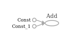 As you can see, each tensor has a unique name (which is comprised of the name of
the name of the node that they come from and the output index at that node, like
this:
 node_name:index), a shape, and a data type. In the example above, the
shape of all of the variables is a scalar, denoted by the empty tuple ().
Note also how the none of the tensors have any values yet. Specifically, the piece of code above did not trigger any addition yet. The actual execution of the computation happens within a session:
with tf.Session() as sess:
    print(sess.run(result))
42
A single session can be reused over and over again to perform more computation.
The first parameter to the run method represents the tensors and operations
that should be evaluated. TensorFlow will then inspect the computational graph
and run all operations that are required to determine the requested value. You
can also pass structured arguments to run to evaluate multiple tensors:
with tf.Session() as sess:
    print(sess.run(x))  # returns a scalar
    print(sess.run([x, y, result]))  # returns a list of scalars
    print(sess.run({"x": x, "my_result": result}))  # returns a dictionary of scalars
8
[8, 34, 42]
{'x': 8, 'my_result': 42}
N.B.: Make sure that you are using sessions in a with construct or
manually close them using session.close() once you do not need them anymore.
Placeholders, Variables, Optimizers
Before we get to the meat of TensorFlow, i.e. building and training deep neural networks, let us take a few minutes to look at three more components that we will be using later on: Placeholders, variables, and optimizers.
Placeholders
Placeholders can be thought of holes in the computation graph, or simply parameters of the computation graph that can be set independently for each run in a session. They are very useful to represent inputs to a computation. We could, for example, parametrize our example from above to add arbitrary numbers instead of hard-coded constants:
x = tf.placeholder(name="x", dtype=tf.float32)  # almost anything in TensorFlow can be named.
y = tf.placeholder(name="y", dtype=tf.float32)
result = x + y  # the common operations for tensors are available as operators

print(x)
print(y)
print(result)
Tensor("x:0", dtype=float32)
Tensor("y:0", dtype=float32)
Tensor("add:0", dtype=float32)
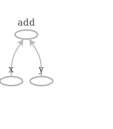
The actual values of the placeholders are filled in at runtime like so:
with tf.Session() as sess:
    # Add up 8 and 34
    result_value = sess.run(result, feed_dict={x: 8, y: 34})
    print("8 + 34 = %d" % result_value)

    # We didn't specify the shapes of our placeholders above, so we can substitute in anything
    # that can be added up!
    feed_dict = {
        x: np.arange(12).reshape(3, 4),
        y: np.ones(12).reshape(3, 4) * 10
    }
    result_value = sess.run(result, feed_dict)
    print("Sum of two 3x4 matrices:\n" + str(result_value))
8 + 34 = 42
Sum of two 3x4 matrices:
[[ 10.  11.  12.  13.]
 [ 14.  15.  16.  17.]
 [ 18.  19.  20.  21.]]
Variables
Variables are stateful elements in the graph, i.e., they store their values
across multiple calls to run within a session. This is useful to keep track of
the number of steps that have been executed in an optimization or to store
weights that change over the course of optimization (e.g. weights of a neural
network).
In TensorFlow, variables must be initialized to some value before running a session. Therefore, each variable has its own variable initializer. By default, this is a uniformly random initialization.
In the following, we will use a variable to keep a running sum over all inputs that we have seen. Keep the analogy to writing a program vs. executing it in mind when reading the following cell:
a = tf.placeholder(name="a", shape=(2, 2), dtype=tf.float32)  # our input are 1x2 matrices

# create the variable and specify that it should be initialized with zeros
accumulator = tf.get_variable(name="acc",
                              shape=(2, 2),
                              dtype=tf.float32,
                              initializer=tf.zeros_initializer())

# compute the new value of the accumulator and assign it to the variable
new_accumulator = accumulator + a
update_accumulator = tf.assign(accumulator, new_accumulator)
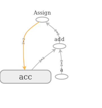
Note that the yellow edge specifies that the assign operation references the
accumulator acc. The edges in the graph (that is, the tensors) are annotated
with their statically known shapes that we hardcoded into the program.
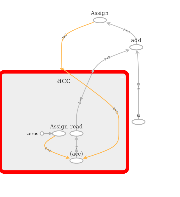
Under the hood, TensorFlow created a bunch of operations and grouped them with
our given name acc. This is typical: TensorFlow provides many primitive
operations, but you will usually use them through abstractions:
We can now run a few steps of the computation:
with tf.Session() as sess:
    sess.run(tf.global_variables_initializer())  # variables need to be initialized before using them!

    # let's look at the initial value of the accumulator:
    print('Initial value of `acc`: \n' + str(sess.run(accumulator)))

    # we can query the value of `new_accumulator` without updating the variable `acc`
    summand = np.random.randn(2, 2)
    feed_dict = {a: summand}
    results = sess.run([new_accumulator, accumulator], feed_dict)
    print('Evaluating `new_accumulator` does not update `acc`: \n' + str(results[1]))

    # but evaluating the assignment does update the accumulator
    for i in range(10):
        summand = np.random.randn(2, 2)
        sess.run(update_accumulator, feed_dict={a: summand})
    print('Evaluating `update_accumulator` updates `acc`: \n' + str(sess.run(accumulator)))
Initial value of `acc`:
[[ 0.  0.]
 [ 0.  0.]]
Evaluating `new_accumulator` does not update `acc`:
[[ 0.  0.]
 [ 0.  0.]]
Evaluating `update_accumulator` updates `acc`:
[[ 3.20579314 -1.38578141]
 [-2.16290545  1.50033629]]
Note that
- variables must be initialized prior to using them and we can specify and initializer for them,
- the assignment is only executed if we explicitly ask for it,
- explicit variable use is most likely not something that you will stumble over regularly.
Optimizers
The last conceptual puzzle piece that we need are optimizers. Optimizers are high-level abstractions in TensorFlow that allow you to perform optimization and automatically adjust variables over the course of a session. Optimizers allow you to minimize a given quantity in your graph using gradient descent and its relatives.
In the following, we will use placeholders, variables, and optimizers to calculate the square-root of an input value using gradient descent.
q = tf.placeholder(name="q", shape=(), dtype=tf.float32)
sqrt_q = tf.get_variable(name="sqrt_q",
                         shape=(),
                         dtype=tf.float32,
                         initializer=tf.ones_initializer())

# Name scopes can be used to group operations together, making it easier to avoid name-clashes
# and making the graph structure easier to understand
with tf.name_scope("error"):
    delta = (q - (sqrt_q * sqrt_q))
    loss = tf.multiply(delta, delta)

# build the optimizer and get a tensor that performs the optimization when evaluated
optimizer = tf.train.GradientDescentOptimizer(name="SGD", learning_rate=0.001)
optimization_step = optimizer.minimize(loss)
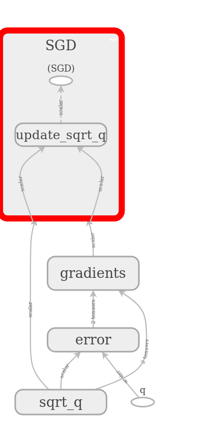
As you can see,
- TensorFlow automatically added operations to compute the gradients for the optimizer,
- the optimizer takes care of updating our variable
sqrt_q, - we neatly grouped the computation of the error, making the graph easy to read.
Let us now run the actual optimization step-by-step until convergence:
def compute_sqrt(x):
    with tf.Session() as sess:
        # Initialize all variables, in our case this sets sqrt_q to 1
        sess.run(tf.global_variables_initializer())

        feed_dict = {
            q: x
        }

        step = 0
        loss_value = 1
        while loss_value > 1e-10:
            # we repeatedly evaluate the optimization step, get the loss, and optimized value
            _, loss_value, sqrt = sess.run((optimization_step, loss, sqrt_q), feed_dict=feed_dict)

            if step % 5 == 0:
                print('Current loss: %f with value %f' % (loss_value, sqrt))
            step += 1

        print('Final loss: %f after %d steps' % (loss_value, step))
        sqrt = sess.run(sqrt_q)
        print('Sqrt of %f is %f' % (x, sqrt))
        return sqrt

compute_sqrt(49)
Current loss: 2304.000000 with value 1.000000
Current loss: 1887.734863 with value 2.356254
Current loss: 688.755493 with value 4.770309
Current loss: 30.682312 with value 6.592484
Current loss: 0.291972 with value 6.961297
Current loss: 0.002077 with value 6.996744
Current loss: 0.000014 with value 6.999729
Current loss: 0.000000 with value 6.999977
Current loss: 0.000000 with value 6.999998
Final loss: 0.000000 after 43 steps
Sqrt of 49.000000 is 7.000000

6.9999995
Of course, there are much better ways to compute the square-root of a number, but the general idea of how to use optimizers has hopefully been made clear :)
Cleaning the Plate
We should now wipe the plate clean before we start with DNNs in TensorFlow: Everything that we did up until now has been added to the same computation graph. The pictures above don’t tell the whole story; it would look rather messy right now. Right now, we should not worry about managing the graph that TensorFlow creates its operations in, but we should return to a clean graph using:
tf.reset_default_graph()
This is mostly necessary when using TensorFlow within a Jupyter notebook, since the default graph would be reset anyway every time you shut down Python.
Your First CNN in TensorFlow
As a slightly more exciting application, we will implement a CNN for MNIST classification, covering the following points:
- defining a CNN,
- loading data from files asynchronously,
- saving the state of the CNN,
- and monitoring the training using TensorBoard.
The part on data loading is absolutely on the bleeding edge, as we will be using TensorFlow’s new Dataset API that was added in version 1.3 and is going to get exciting new features in version 1.4.
Building the Model
By now, you probably have an idea of what it takes to create a CNN in TensorFlow:
- create a placeholder tensor that represents the input,
- define variables for the kernels, weights, and biases of the layers,
- create an optimizer and minimize some loss.
In general, it is a good idea to write a bunch of functions that abstract over some of these steps. Specifically, we will separate the concerns of building the model, training the model, and feeding data into the model. This way we can use the same model for evaluation (needs data streaming, but no optimization), training (needs data streaming and optimization), and deployment (operates on single images, but no optimization).
Building a convolution
Since we will need to define multiple convolutions, we may be tempted to write a function to do that:
def make_convolution(input, name, kernel_size, num_filters, stride, padding='SAME'):

    # We are using a variable scope here to ensure that the `kernel` variable name
    # is taken relative to the name of this convolution.
    with tf.name_scope(name), tf.variable_scope(name):
        # get the number of input channels, assuming NHWC format
        in_channels = input.get_shape()[-1]
        # create the kernel of the convolution
        kernel = tf.get_variable(name="kernel",
                                 shape=[kernel_size, kernel_size, in_channels, num_filters])
        output = tf.nn.conv2d(input,
                              kernel,
                              strides=[1, stride, stride, 1],
                              padding=padding)
        # create bias, choose correct initializers etc.
        return tf.nn.relu(output)
While this is generally possible, the above implementation has multiple issues and it should go without saying that we usually do not need this level of detail. Luckily, these problems have already been solved by other people. There are plenty of libraries around that can be used to make the task of specifying DNNs less painful:
- TF Layers
- TF Slim
- Keras
- …
We will use TFLayers (TFSlim is also a very good choice, especially for larger networks), since it is a somewhat thinner wrapper around TensorFlow than Slim.
The Model Function
def model(input):
    """
        This function creates a CNN with two convolution/pooling pairs, followed by two dense layers.
        These are then used to predict one of ten digit classes.

        Arguments:
            input: a tensor with shape `[batch_size, 28, 28, 1]` representing MNIST data.

        Returns:
            A dictionary with the keys `probabilities`, `class`, and `logits`, containing the
            corresponding tensors.
    """

    # we assume the input has shape [batch_size, 28, 28, 1]
    net = input

    # create two convolution/pooling layers
    for i in range(1, 3):
        net = tf.layers.conv2d(inputs=net,
                               filters=32 * i,
                               kernel_size=[5, 5],
                               padding="same",
                               activation=tf.nn.relu,
                               name="conv2d_%d" % i)
        net = tf.layers.max_pooling2d(inputs=net,
                                      pool_size=[2, 2],
                                      strides=2,
                                      name="maxpool_%d" % i)
    # flatten the input to [batch_size, 7 * 7 * 64]
    net = tf.reshape(net, [-1, 7 * 7 * 64])
    net = tf.layers.dense(net, units=128, name="dense_1")
    logits = tf.layers.dense(net, units=10, name="dense_2")
    # logits has shape [batch_size, 10]

    # The predictions of our model; we return the logits to formulate a numerically
    # stable loss in our optimization routine
    tensors = {
        "probabilities": tf.nn.softmax(logits),
        "class": tf.argmax(logits, axis=-1),
        "logits": logits
    }
    return tensors
This is the core of the model. We could now use it like this:
def classify_image(img):
    input_image = tf.placeholder(...)
    outputs = model(input_image)
    with tf.Session() as sess:
        # initialize model etc. ...
        return sess.run(outputs["class"], feed_dict: {input_image: img})
But the strength of this approach is that we can also use different ways to feed images to the model. Before we get to that, we need to define an optimizer and the corresponding loss:
def training_model(input, label):
    tensors = model(input)
    logits = tensors["logits"]

    # one-hot encode the labels, compute cross-entropy loss, average
    # over the number of elements in the mini-batch
    with tf.name_scope("loss"):
        label = tf.one_hot(label, 10)
        loss = tf.nn.softmax_cross_entropy_with_logits(labels=label, logits=logits)
        loss = tf.reduce_mean(loss)
    tensors["loss"] = loss

    # create the optimizer and register the global step counter with it,
    # it is increased every time the optimization step is executed
    optimizer = tf.train.AdamOptimizer(learning_rate=1e-3)
    global_step = tf.train.get_or_create_global_step()
    tensors["opt_step"] = optimizer.minimize(loss, global_step=global_step)
    return tensors
We are almost there now. The only thing to create a proper training procedure is data. The next part deals with loading data, but feel free to skip any details.
Loading Data
Starting with version 1.3, TensorFlow ships with a powerful dataset API that allows you to quickly manipulate and load datasets with multi-threading support. The API’s design has a functional flavor and should be familiar to anyone who has programmed with LINQ in C#, Haskell, or another functional programming language. A dataset can then be thought of as a process producing data points sequentially.
Our data is split in testing and training data. Each digit class has its own subfolder in which each image is stored as a PNG file. For both training and testing sets, a file containing a list of the relative paths to all of these files has been created. We will proceed as follows:
- In Python code, we will read that list, construct the labels from it, and shuffle them once
- Using the dataset API, we construct a dataset from the list of datapoints by
splitting it into two lists and calling
Dataset.from_tensor_sliceson it. - This dataset now contains pairs of relative file paths and class labels. These are already tensors, and from here on no Python code will touch this data during runtime.
- For training, this dataset is repeated indefinitely (
repeat(-1)) and shuffled again internally by randomly picking one of the next 10000 data points (shuffle(10000)) - In all cases, we use
Dataset.mapto apply an operation to each element of the dataset: In our case, this operation reads the file at the given path, decodes it as a PNG, and casts it to a float. Note that the call ismap(read_image), butread_imagehere is only the Python function that constructs the operation that is applied to each image. Note also that we are using 4 threads to load the images in parallel and keep up to100 * batch_sizemany images ready. - For the training dataset, we batch the specified number of datapoints
For MNIST, this is of course overkill, since the dataset would actually fit into memory in its entirety. Also, if this approach here is used, it would probably be faster to not load the list-file into memory at once: Either use a file format that is able to store not only the images but also the labels, or reconstruct the labels from the file paths using pure TensorFlow code at run time.
def load_data_set(is_training=True):
    """
        Loads either the training or evaluation dataset by performing the following steps:
        1. Read the file containing the file paths of the images.
        2. Construct the correct labels from the file paths.
        3. Shuffle paths jointly with the labels.
        4. Turn them into a dataset of tuples.

        Arguments:
            is_training: whether to load the training dataset or the evaluation dataset

        Returns:
            The requested dataset as a dataset containing tuples `(relative_path, label)`.
    """
    substring = "training" if is_training else "testing"
    file = "mnist_%s.dataset" % substring

    # this converts the file names into (file_name, class) tuples
    offset = len('mnist_data/%s/c' % substring)
    data_points = []
    with open(file, 'r') as f:
        for line in f:
            cls = int(line[offset])
            path = abspath(line.strip())
            data_points.append((path, cls))

    # now shuffle all data points around and create a dataset from it
    from random import shuffle
    shuffle(data_points)

    # Neat fact: zip can be used to build its own inverse:
    data_points = zip(*data_points)

    # note how this is a tensor of strings! Tensors are not inherently numeric!
    images = tf.constant(data_points[0])
    labels = tf.constant(data_points[1])

    # `from_tensor_slices` takes a tuple of tensors slices them along the first
    # dimension. Thus we get a dataset of tuples.
    return tf.contrib.data.Dataset.from_tensor_slices((images, labels))

def read_image(img_path, label):
    """
        Constructs operations to turn the path to an image to the actual image data.

        Arguments:
            img_path: The path to the image.
            label: The label for the image.

        Returns:
            A tuple `(img, label)`, where `img` is the loaded image.
    """
    img_content = tf.read_file(img_path)
    img = tf.image.decode_png(img_content, channels=1)
    img = tf.image.convert_image_dtype(img, tf.float32)
    return img, label

def make_training_dataset(batch_size=128):
    """
        Creates a training dataset with the given batch size.
    """
    dataset = load_data_set(is_training=True)
    dataset = dataset.repeat(-1)
    dataset = dataset.shuffle(10000)
    dataset = dataset.map(read_image,
                          num_threads=4,
                          output_buffer_size=100 * batch_size)
    dataset = dataset.batch(batch_size)
    return dataset

def make_eval_dataset(batch_size=128):
    """
        Creates the evaluation dataset.
    """
    dataset = load_data_set(is_training=False)
    dataset = dataset.map(read_image,
                          num_threads=4,
                          output_buffer_size=100 * batch_size)
    dataset = dataset.batch(batch_size)
    return dataset
Training the Model
Finally, we get to train the model. Most of the steps should be familiar by now.
Note here how the dataset is accessed: We create an iterator from the dataset
and call get_next on it to receive a tuple of tensors that represent the next
images and labels of the input. Again, calling get_next does not execute
anything: Only by passing these tensors to the model we force their evaluation
when the model is run, which is when the data is actually fetched from the input
dataset.
def perform_training(steps, batch_size):
    dataset = make_training_dataset(batch_size)
    # The one-shot iterator is just another node in the graph, and so is the
    # `get_next` operation. The tensors produced by `get_next` depend on the
    # structure of the dataset that we build: Our dataset consists of tuples,
    # so we get a tuple of tensors.
    next_image, next_label = dataset.make_one_shot_iterator().get_next()
    model_outputs = training_model(next_image, next_label)

    loss = model_outputs["loss"]
    opt_step = model_outputs["opt_step"]
    with tf.Session() as sess:
        sess.run(tf.global_variables_initializer())

        for i in xrange(steps):
            # Note how we no longer need to use the `feed_dict`. This avoids
            # additional overhead due to Python -> native Tensorflow
            # serialization
            _, loss_value = sess.run((opt_step, loss))

            if i % 5 == 0:
                print("Loss: %f" % loss_value)
        print("Final Loss: %f" % loss_value)
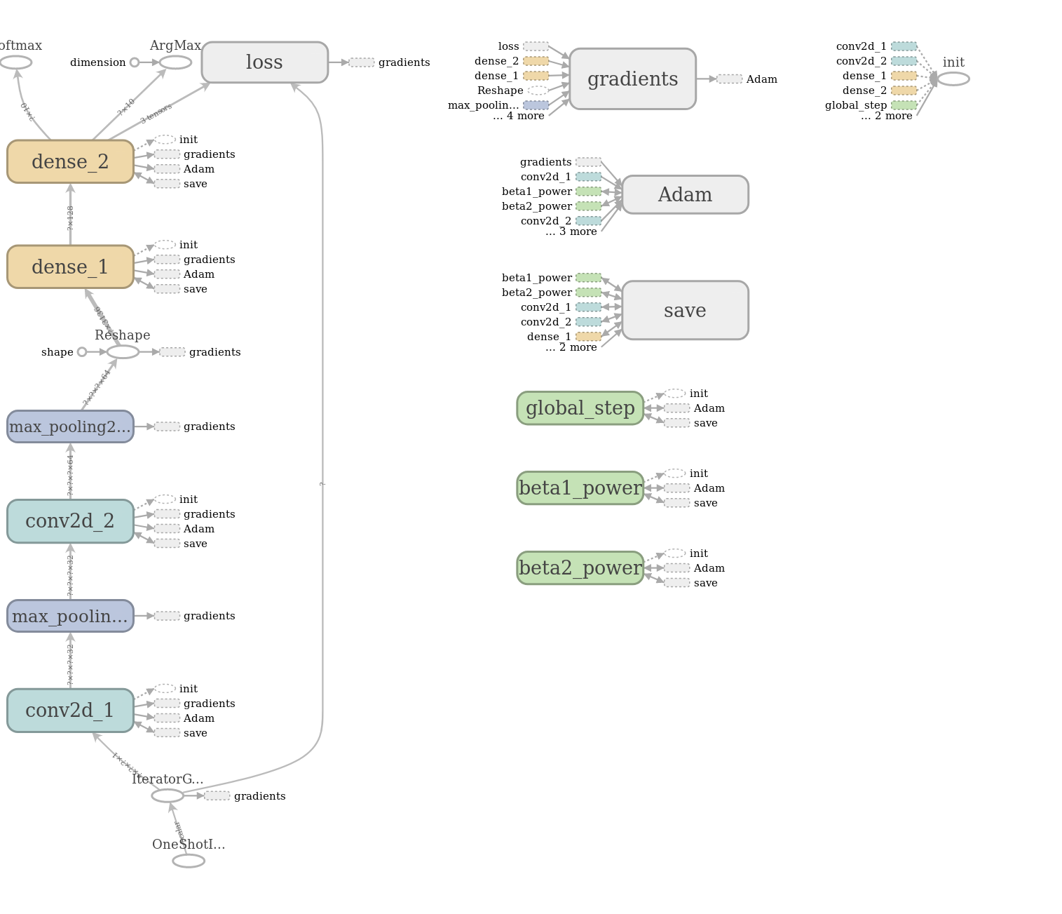
We can now train the model for a few steps and watch the loss go down. I have
added a bit of visualization code to the perform_training function from above,
so the signature has changed slightly, but the code is essentially the same:
tutorial.perform_training_with_visualization(steps=500, batch_size=128,
                                             dataset=make_training_dataset,
                                             model=training_model)
<IPython.core.display.Javascript object>
Final Loss: 0.059373
Saving and Loading Models
The training code form above still has an obvious problem: It does not save the weights it has learned. Once the session is closed, all variables are lost. TensorFlow models are stored in two parts:
-
You can save the whole computation graph as a metagraph file. This writes the structure of the computation graph into a file that can be reimported later. If you are familiar with caffe: This corresponds to saving a protobuf definition of your network. I generally want to discourage this: Instead of saving the metagraph, save the Python code that creates your model. Metagraphs are stored as binary protobufs, which makes them hard to read for humans, and even harder to modify. Avoid getting into a situation in which a metagraph is the only way to rebuild the computation graph of your model. If you are still interested in metagraphs, check the TensorFlow documentation.
-
The values of variables of a model can be saved in a checkpoint. This is what we will be using to store the state of our model. By default, all variables in your model’s graph are saved, but you can also select a subset. Generally, what you need to save depends on your use-case: If you are storing a checkpoint to resume training later on, you will want to also save the variables introduced by the optimizer. If you are storing a checkpoint to load it for inference, you can drop all of that.
Saving a checkpoint for a model works by using tf.train.Saver and its
associated save and restore methods:
    saver = tf.train.Saver(variables_to_save)
    with tf.Session() as sess:
        sess.run(tf.global_variables_initializer())
        saver.restore(sess, "checkpoint-file-to-restore-from")
        # your code here
        saver.save(sess, "checkpoint-file-to-save-to")
Here is a revised training method that supports saving. It uses
get_variables_for_saver from the accompanying tutorial.py file to filter the
variables of the model according to regular expressions.
def perform_training(steps, batch_size, checkpoint_name):
    dataset = make_training_dataset(batch_size)
    next_image, next_label = dataset.make_one_shot_iterator().get_next()
    model_outputs = training_model(next_image, next_label)

    loss = model_outputs["loss"]
    opt_step = model_outputs["opt_step"]

    # We exclude some variables created by the optimizer and data loading process
    # when saving the model, since we assume that we do not want to continue training
    # from the checkpoint.
    variables_to_save = tutorial.get_variables_for_saver(exclude=[".*Adam", ".*beta", ".*Iterator"])
    saver = tf.train.Saver(variables_to_save)
    with tf.Session() as sess:
        sess.run(tf.global_variables_initializer())

        for i in xrange(steps):
            _, loss_value = sess.run((opt_step, loss))

        # In the end, we  will save the model
        saver.save(sess, checkpoint_name)
        print("Final Loss: %f" % loss_value)


tf.reset_default_graph()
perform_training(steps=100, batch_size=128,
                 checkpoint_name="model")
Final Loss: 0.060810
Building an Image Classifier
This can now be used to build an image classifier that takes the name of the checkpoint with the variables and a list of images (as numpy arrays) and maps them to a list of predictions:
def image_classifier(checkpoint_name, *images):
    # note that we are deciding to feed the images one-by-one for simplicity
    input = tf.placeholder(name="input", shape=(1, 28, 28, 1), dtype="float32")
    tensors = model(input)

    saver = tf.train.Saver()
    with tf.Session() as sess:
        # Initialize all variables, since there may be variables in our graph that aren't
        # loaded form the checkpoint
        sess.run(tf.global_variables_initializer())
        saver.restore(sess, checkpoint_name)

        classes = []
        for i in images:
            cls = sess.run(tensors["class"], feed_dict={input: np.expand_dims(i, 0)})
            classes.append(cls[0])
        return classes
Let’s give it a shot:
def load_image_as_array(filepath):
    im = Image.open(abspath(filepath)).convert('L')
    (width, height) = im.size
    greyscale_map = list(im.getdata())
    greyscale_map = np.array(greyscale_map)
    greyscale_map = greyscale_map.reshape((height, width, 1))
    return greyscale_map


tf.reset_default_graph()
images = [
    "mnist_data/testing/c1/994.png",
    "mnist_data/testing/c8/606.png",
    "mnist_data/testing/c4/42.png"
]
classification = image_classifier("model", *map(load_image_as_array, images))
print("Classification: " + str(classification))
INFO:tensorflow:Restoring parameters from model
Classification: [1, 8, 4]
This is probably not the best way to turn this into a classifier for deployment, but absolutely sufficient for development environments. There is detailed documentation available on what is the proper way to do this, see for example the TensorFlow Serving documentation.
A Very Basic Evaluation
With all of this, we can build a minimal evaluation script that loads the weights and keeps track of some metrics. Tensorflow comes with support for some metrics, making it easy to track them. We can write a simple wrapper around our model that tracks
- accuracy,
- number of false negatives, and
- number of false positives. Each metric consists of an operation to update the metric and a tensor that represents the value of the metric. The update-operation needs to be run in each step of the evaluation.
def evaluation_model(input, label):
    tensors = model(input)
    # Let's track some metrics like accuracy, false negatives, and false positives.
    # Each of them returns a tuple `(value, update_op)`. The value is, well, the value
    # of the metric, the update_op is the tensor that needs to be evaluated to update
    # the metric.
    accuracy, update_acc = tf.metrics.accuracy(label, tensors["class"])
    false_negatives, update_fn = tf.metrics.false_negatives(label, tensors["class"])
    false_positives, update_fp = tf.metrics.false_positives(label, tensors["class"])
    tensors["accuracy"] = accuracy
    tensors["false_negatives"] = false_negatives
    tensors["false_positives"] = false_positives
    # We can group the three metric updates into a single operation and run that instead.
    tensors["update_metrics"] = tf.group(update_acc, update_fn, update_fp)
    return tensors
Running the evaluation is very similar to running the training, but
- it uses the evaluation model and dataset,
- it loads the checkpoint created in the training procedure to get the correct weights,
- instead of running the optimization operation, it just updates the metrics,
- it only goes over the input dataset once and stop once we processed all samples,
- it outputs the metrics in the end.
def perform_evaluation(checkpoint_name):
    # this is the same as in the training case, except that we are using the
    # evaluation dataset and model
    dataset = make_eval_dataset()
    next_image, next_label = dataset.make_one_shot_iterator().get_next()
    model_outputs = evaluation_model(next_image, next_label)

    saver = tf.train.Saver()
    with tf.Session() as sess:
        # Initialize variables. This is really necessary here since the metrics
        # need to be initialized to sensible values. They are local variables,
        # meaning that they are not saved by default, which is why we need to run
        # `local_variables_initializer`.
        sess.run(tf.global_variables_initializer())
        sess.run(tf.local_variables_initializer())
        # restore the weights
        saver.restore(sess, checkpoint_name)

        update_metrics = model_outputs["update_metrics"]
        # feed the inputs until we run out of images
        while True:
            try:
                _ = sess.run(update_metrics)
            except tf.errors.OutOfRangeError:
                # this happens when the iterator runs out of samples
                break

        # Get the final values of the metrics. Note that this call does not access the
        # `get_next` node of the dataset iterator, since these tensors can be evaluated
        # on their own and therefore don't cause the exception seen above to be triggered
        # again.
        accuracy = model_outputs["accuracy"]
        false_negatives = model_outputs["false_negatives"]
        false_positives = model_outputs["false_positives"]
        acc, fp, fn = sess.run((accuracy, false_negatives, false_positives))
        print("Accuracy: %f" % acc)
        print("False positives: %d" % fp)
        print("False negatives: %d" % fn)


tf.reset_default_graph()
perform_evaluation(checkpoint_name="model")
INFO:tensorflow:Restoring parameters from model
Accuracy: 0.963600
False positives: 39
False negatives: 10
Monitoring Training and Visualizing Your Model
For the training in this notebook, we used a custom visualization using
pyplot. Tensorflow comes with its own tools that help you to monitor the
training process and visualize the computation graph (this is also what was used
to generate the graph drawings in this notebook).
There are two steps to monitoring your model:
- Change the training script to create summaries of all the variables you want
to keep track of. All the relevant functions for this live in
tensorflow.summary. For exampletensorflow.summary.scalar(name, tensor)returns a tensor that when executed creates a summary that can be logged into what is known as an event file. As such, the summary tensors must be evaluated periodically and their results written to file. - Open TensorBoard to access the summaries from a web-interface.
For the first step, we will modify the training procedure such that we have two different summary operations that are executed from time to time: In every training step, we will keep a summary of the log. Additionally, we will write out the input image and histograms of the softmax distribution and the logit activations every few steps.
def perform_training(steps, batch_size, checkpoint_name, logdir):
    dataset = make_training_dataset(batch_size)
    next_image, next_label = dataset.make_one_shot_iterator().get_next()
    model_outputs = training_model(next_image, next_label)

    loss = model_outputs["loss"]
    opt_step = model_outputs["opt_step"]

    # generate summary tensors, but don't store them -- there's a better way
    frequent_summary = tf.summary.scalar("loss", loss)
    tf.summary.histogram("logits", model_outputs["logits"])
    tf.summary.histogram("probabilities", model_outputs["probabilities"])
    # only log one of the `batch_size` many images
    tf.summary.image("input_image", next_image, max_outputs=1)

    # merge all summary ops into a single operation
    infrequent_summary = tf.summary.merge_all()

    variables_to_save = tutorial.get_variables_for_saver(exclude=[".*Adam", ".*beta", ".*Iterator"])
    saver = tf.train.Saver(variables_to_save)

    # the summary writer will write the summaries to the specified log directory
    summary_writer = tf.summary.FileWriter(logdir=logdir, graph=tf.get_default_graph())
    with tf.Session() as sess:
        sess.run(tf.global_variables_initializer())

        for i in xrange(steps):
            # note that we explicitly ask for the evaluation of the summary ops
            if i % 10 == 0:
                _, summary = sess.run((opt_step, infrequent_summary))
            else:
                _, summary = sess.run((opt_step, frequent_summary))
            # ...and we also need to explicitly add them to the summary writer
            summary_writer.add_summary(summary, global_step=i)

        saver.save(sess, checkpoint_name)
        summary_writer.close()


tf.reset_default_graph()
# It's a good idea to keep the checkpoint and the event files in the same directory
perform_training(steps=5000,
                 batch_size=128,
                 checkpoint_name="training/model",
                 logdir="training")

tf.reset_default_graph()
perform_evaluation(checkpoint_name="training/model")
INFO:tensorflow:Restoring parameters from training/model
Accuracy: 0.991700
False positives: 7
False negatives: 3
To view the data, run TensorBoard and point it to the right directory:
tensorboard --logdir training, in our case.
TensorBoard live demo here!
What Next?
If you are interested, I would be willing to prepare another session on multi- GPU training with TensorFlow. This would most likely also cover some topics like how to use the currently available profiling tools and whatever questions you would like to get answers to.
Further Reading
TensorFlow comes with a plethora of libraries that make life easier:
tf.imagehas functions that can be used for loading and augmenting imagestf.contribcontains all kinds of contributed code that is still subject to changetf.distributionscontains code for sampling within your modelstf.estimatorcontains the Estimators API, which allows to quickly create, train, and execute models with a SciKitLearn-like interfacetf.lossescontains common loss functionstf.nncontains functions that are suitable to build neural networks from scratchtf.profilercontains profiling tools for TensorFlow models; these are still in development but can already give you some good insights into what your model is doingtf.traincontains many features that take a high-level approach to training models. Take a look atMonitoredTrainingSession, which automates checkpoint saving, writing summaries, failure handling, etc.tf.contrib.datacontains the dataset API that we have been using in this notebook. This API is under very active development and should get even better over time :)